(Authors: Prof. Navdeep M. Singh, VJTI, University of Mumbai and Nalin Pithwa, 1992).
Abstract: The bilinear transformation can be achieved by using the method of synthetic division. A good deal of simplification is obtained when the process is implemented as a sequence of matrix operations. Besides, the matrices are found to have simple structures suitable for algorithmic implementation.
I) INTRODUCTION:
Davies [1] proposed a method for bilinear transformation using synthetic division. This method can be quite simplified when the synthetic division is carried out as a set of matrix operations because the operator matrices are found to have simple structures and so can be easily generated.
II) THE ALGORITHM:
Given a discrete time transfer function 


This can be sequentially achieved as :-

The first step is to represent the given characteristic polynomial in the standard companion form. Since the companion form represents a monic polynomial appropriate scaling is required in the course of the algorithm to ensure that the polynomial generated is monic after each step of transformation.
The method is developed for a third degree polynomial and then generalized.
Step 1:

Given 
Then, 


In the companion form, obviously the following transformation is sought:
![A = \left[ \begin{array}{ccc} 0 & 1 & 0 \\ 0 & 0 & 1 \\ -a_{0} & -a_{1} & -a_{2} \end{array}\right]](https://s0.wp.com/latex.php?latex=A+%3D+%5Cleft%5B+%5Cbegin%7Barray%7D%7Bccc%7D+0+%26+1+%26+0+%5C%5C+0+%26+0+%26+1+%5C%5C+-a_%7B0%7D+%26+-a_%7B1%7D+%26+-a_%7B2%7D+%5Cend%7Barray%7D%5Cright%5D&bg=ffffff&fg=333A42&s=0&c=20201002)
![B=\left[ \begin{array}{ccc} 0 & 1 & 0 \\ 0 & 0 &1 \\-b_{0} & -b_{1} & -b_{2} \end{array} \right]](https://s0.wp.com/latex.php?latex=B%3D%5Cleft%5B+%5Cbegin%7Barray%7D%7Bccc%7D+0+%26+1+%26+0+%5C%5C+0+%26+0+%261+%5C%5C-b_%7B0%7D+%26+-b_%7B1%7D+%26+-b_%7B2%7D+%5Cend%7Barray%7D+%5Cright%5D&bg=ffffff&fg=333A42&s=0&c=20201002)
![C = \left[ \begin{array}{ccc} 0 & 1 & 0 \\ 0 & 0 & 1 \\ -a_{0}-a_{1}-a_{2}-1 & -a_{1} - 2a_{2}-3 & -a_{2}-3 \end{array} \right]](https://s0.wp.com/latex.php?latex=C+%3D+%5Cleft%5B+%5Cbegin%7Barray%7D%7Bccc%7D+0+%26+1+%26+0+%5C%5C+0+%26+0+%26+1+%5C%5C+-a_%7B0%7D-a_%7B1%7D-a_%7B2%7D-1+%26+-a_%7B1%7D+-+2a_%7B2%7D-3+%26+-a_%7B2%7D-3+%5Cend%7Barray%7D+%5Cright%5D&bg=ffffff&fg=333A42&s=0&c=20201002)
Performing elementary row and column transformations on A using matrix operators, the final row operator and column operator matrices, 

![P_{1} = \left[ \begin{array}{ccc} (a_{0}+a_{1})/a_{0} & a_{2}/a_{0} & 1/a_{0} \\ -1 & 1 & 0 \\ 0 & -1 & 1\end{array} \right]](https://s0.wp.com/latex.php?latex=P_%7B1%7D+%3D+%5Cleft%5B+%5Cbegin%7Barray%7D%7Bccc%7D+%28a_%7B0%7D%2Ba_%7B1%7D%29%2Fa_%7B0%7D+%26+a_%7B2%7D%2Fa_%7B0%7D+%26+1%2Fa_%7B0%7D+%5C%5C+-1+%26+1+%26+0+%5C%5C+0+%26+-1+%26+1%5Cend%7Barray%7D+%5Cright%5D&bg=ffffff&fg=333A42&s=0&c=20201002)
![Q_{1} = \left[ \begin{array}{ccc} 1 & 0 & 0 \\ 1 & 1 & 0 \\ 1 & 1 & 1 \end{array}\right]](https://s0.wp.com/latex.php?latex=Q_%7B1%7D+%3D+%5Cleft%5B+%5Cbegin%7Barray%7D%7Bccc%7D+1+%26+0+%26+0+%5C%5C+1+%26+1+%26+0+%5C%5C+1+%26+1+%26+1+%5Cend%7Barray%7D%5Cright%5D&bg=ffffff&fg=333A42&s=0&c=20201002)
Thus, 
In general, for a polynomial of degree n,
![P_{1} = \left[ \begin{array}{ccccc} (a_{0}+a_{1})/a_{0} & a_{2}/a_{0} & a_{3}/a_{0} & \ldots & 1\\ -1 & 1 & 0 & \ldots & a_{0}\\ 0 & -1 & 1 & \ldots & 0 \\ \vdots & \vdots & \vdots & \vdots & \vdots \\ \vdots & \vdots & \vdots & -1 & 1\end{array}\right]](https://s0.wp.com/latex.php?latex=P_%7B1%7D+%3D+%5Cleft%5B+%5Cbegin%7Barray%7D%7Bccccc%7D+%28a_%7B0%7D%2Ba_%7B1%7D%29%2Fa_%7B0%7D+%26+a_%7B2%7D%2Fa_%7B0%7D+%26+a_%7B3%7D%2Fa_%7B0%7D+%26+%5Cldots+%26+1%5C%5C+-1+%26+1+%26+0+%26+%5Cldots+%26+a_%7B0%7D%5C%5C+0+%26+-1+%26+1+%26+%5Cldots+%26+0+%5C%5C+%5Cvdots+%26+%5Cvdots+%26+%5Cvdots+%26+%5Cvdots+%26+%5Cvdots+%5C%5C+%5Cvdots+%26+%5Cvdots+%26+%5Cvdots+%26+-1+%26+1%5Cend%7Barray%7D%5Cright%5D&bg=ffffff&fg=333A42&s=0&c=20201002)
![Q_{1} = \left[ \begin{array}{ccccc} 1 & 0 & 0 \ldots & 0 \\ 1 & 1 & 0 & \ldots & \ldots \\ 1 & 1 & 1 & \ldots & \ldots \\ \vdots & \vdots & \vdots & \vdots & \vdots \\ 1 & 1 & 1 & \ldots & 1\end{array}\right]](https://s0.wp.com/latex.php?latex=Q_%7B1%7D+%3D+%5Cleft%5B+%5Cbegin%7Barray%7D%7Bccccc%7D+1+%26+0+%26+0+%5Cldots+%26+0+%5C%5C+1+%26+1+%26+0+%26+%5Cldots+%26+%5Cldots+%5C%5C+1+%26+1+%26+1+%26+%5Cldots+%26+%5Cldots+%5C%5C+%5Cvdots+%26+%5Cvdots+%26+%5Cvdots+%26+%5Cvdots+%26+%5Cvdots+%5C%5C+1+%26+1+%26+1+%26+%5Cldots+%26+1%5Cend%7Barray%7D%5Cright%5D&bg=ffffff&fg=333A42&s=0&c=20201002)

and ![B = P_{1}AQ_{1} = \left[ \begin{array}{ccccc} 0 & 1 & 0 & \ldots & 0\\ 0 & 0 & 1 & \ldots & 0 \\ \vdots & \vdots & \vdots & \vdots & \vdots \\ \ldots & \ldots & \ldots & \ldots & \ldots \\ -b_{0} & -b_{1} & -b_{2} & \ldots & -b_{n-1} \end{array}\right]](https://s0.wp.com/latex.php?latex=B+%3D+P_%7B1%7DAQ_%7B1%7D+%3D+%5Cleft%5B+%5Cbegin%7Barray%7D%7Bccccc%7D+0+%26+1+%26+0+%26+%5Cldots+%26+0%5C%5C+0+%26+0+%26+1+%26+%5Cldots+%26+0+%5C%5C+%5Cvdots+%26+%5Cvdots+%26+%5Cvdots+%26+%5Cvdots+%26+%5Cvdots+%5C%5C+%5Cldots+%26+%5Cldots+%26+%5Cldots+%26+%5Cldots+%26+%5Cldots+%5C%5C+-b_%7B0%7D+%26+-b_%7B1%7D+%26+-b_%7B2%7D+%26+%5Cldots+%26+-b_%7Bn-1%7D+%5Cend%7Barray%7D%5Cright%5D&bg=ffffff&fg=333A42&s=0&c=20201002)
Where 

Now, the transformation 


![P_{c1} = \left[ \begin{array}{ccc} 1 & 0 & 0 \\ -1 & 1 & 0 \\ 1 & -2 & 1 \end{array}\right]](https://s0.wp.com/latex.php?latex=P_%7Bc1%7D+%3D+%5Cleft%5B+%5Cbegin%7Barray%7D%7Bccc%7D+1+%26+0+%26+0+%5C%5C+-1+%26+1+%26+0+%5C%5C+1+%26+-2+%26+1+%5Cend%7Barray%7D%5Cright%5D&bg=ffffff&fg=333A42&s=0&c=20201002)
![Q_{c1} = \left[ \begin{array}{ccc} 1 & 0 & 0 \\ 0 & 1 & 0 \\ 0 & 1 & 1 \end{array}\right]](https://s0.wp.com/latex.php?latex=Q_%7Bc1%7D+%3D+%5Cleft%5B+%5Cbegin%7Barray%7D%7Bccc%7D+1+%26+0+%26+0+%5C%5C+0+%26+1+%26+0+%5C%5C+0+%26+1+%26+1+%5Cend%7Barray%7D%5Cright%5D&bg=ffffff&fg=333A42&s=0&c=20201002)
![P_{c1} = \left[ \begin{array}{ccccc}1 & 0 & \ldots & \ldots & 0 \\ -1 & 1 & \ldots & \ldots & 0 \\ 1 & -2 & 1 & \ldots & 0 \\ -1 & 3 & -3 & 1 & \ldots \\ \vdots & \vdots & \vdots & \vdots & \vdots \\ \ldots & \ldots & \ldots & \ldots & 1\end{array}\right]](https://s0.wp.com/latex.php?latex=P_%7Bc1%7D+%3D+%5Cleft%5B+%5Cbegin%7Barray%7D%7Bccccc%7D1+%26+0+%26+%5Cldots+%26+%5Cldots+%26+0+%5C%5C+-1+%26+1+%26+%5Cldots+%26+%5Cldots+%26+0+%5C%5C+1+%26+-2+%26+1+%26+%5Cldots+%26+0+%5C%5C+-1+%26+3+%26+-3+%26+1+%26+%5Cldots+%5C%5C+%5Cvdots+%26+%5Cvdots+%26+%5Cvdots+%26+%5Cvdots+%26+%5Cvdots+%5C%5C+%5Cldots+%26+%5Cldots+%26+%5Cldots+%26+%5Cldots+%26+1%5Cend%7Barray%7D%5Cright%5D&bg=ffffff&fg=333A42&s=0&c=20201002)
![Q_{c1} = \left[ \begin{array}{ccccc} 1 & 0 & \ldots & \ldots & 0 \\ 0 & 1 & 0 & \ldots & 0 \\ 0 & 1 & 1 & \ldots & 0 \\ 0 & 1 & 2 & 1 &\ldots \\ \vdots & \vdots & \vdots & \vdots & \vdots \\ \ldots & \ldots & \ldots & \ldots & 1\end{array}\right]](https://s0.wp.com/latex.php?latex=Q_%7Bc1%7D+%3D+%5Cleft%5B+%5Cbegin%7Barray%7D%7Bccccc%7D+1+%26+0+%26+%5Cldots+%26+%5Cldots+%26+0+%5C%5C+0+%26+1+%26+0+%26+%5Cldots+%26+0+%5C%5C+0+%26+1+%26+1+%26+%5Cldots+%26+0+%5C%5C+0+%26+1+%26+2+%26+1+%26%5Cldots+%5C%5C+%5Cvdots+%26+%5Cvdots+%26+%5Cvdots+%26+%5Cvdots+%26+%5Cvdots+%5C%5C+%5Cldots+%26+%5Cldots+%26+%5Cldots+%26+%5Cldots+%26+1%5Cend%7Barray%7D%5Cright%5D&bg=ffffff&fg=333A42&s=0&c=20201002)
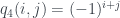
![P_{c1}(i,j) = [|P_{c1(i-j)}|+|P_{c1}(i-1,j-1)|] \times (-1)^{(i+j)}](https://s0.wp.com/latex.php?latex=P_%7Bc1%7D%28i%2Cj%29+%3D+%5B%7CP_%7Bc1%28i-j%29%7D%7C%2B%7CP_%7Bc1%7D%28i-1%2Cj-1%29%7C%5D+%5Ctimes+%28-1%29%5E%7B%28i%2Bj%29%7D&bg=ffffff&fg=333A42&s=0&c=20201002)


Similarly,


Thus, when A is the companion form of a polynomial of any degree n, then 

Step 2:

Let 


The scaling of the entire polynomial by 
The following transformation is sought:
![C = \left[ \begin{array}{ccc} 0 & 1 & 0 \\ 0 & 0 & 1 \\ -b_{0} & -b_{1} & -b_{2} \end{array}\right] \rightarrow D = \left[\begin{array}{ccc} 0 & 1 & 0\\ 0 & 0 & 1 \\ -1/b_{0} & (-b_{2}/b_{0}) & (-b_{1}/b_{0})\end{array}\right]](https://s0.wp.com/latex.php?latex=C+%3D+%5Cleft%5B+%5Cbegin%7Barray%7D%7Bccc%7D+0+%26+1+%26+0+%5C%5C+0+%26+0+%26+1+%5C%5C+-b_%7B0%7D+%26+-b_%7B1%7D+%26+-b_%7B2%7D+%5Cend%7Barray%7D%5Cright%5D+%5Crightarrow+D+%3D+%5Cleft%5B%5Cbegin%7Barray%7D%7Bccc%7D+0+%26+1+%26+0%5C%5C+0+%26+0+%26+1+%5C%5C+-1%2Fb_%7B0%7D+%26+%28-b_%7B2%7D%2Fb_%7B0%7D%29+%26+%28-b_%7B1%7D%2Fb_%7B0%7D%29%5Cend%7Barray%7D%5Cright%5D&bg=ffffff&fg=333A42&s=0&c=20201002)
The row and column operator matrices 

![P_{2}=\left[\begin{array}{ccc} b_{1}/b_{2} & 0 & 0 \\ 0 & b_{2}/b_{1} & 0 \\ 0 & 0 & 1/b_{0}\end{array}\right]](https://s0.wp.com/latex.php?latex=P_%7B2%7D%3D%5Cleft%5B%5Cbegin%7Barray%7D%7Bccc%7D+b_%7B1%7D%2Fb_%7B2%7D+%26+0+%26+0+%5C%5C+0+%26+b_%7B2%7D%2Fb_%7B1%7D+%26+0+%5C%5C+0+%26+0+%26+1%2Fb_%7B0%7D%5Cend%7Barray%7D%5Cright%5D&bg=ffffff&fg=333A42&s=0&c=20201002)
![Q_{2} = \left[ \begin{array} {ccc}1/b_{0} & 0 & 0 \\ 0 & b_{2}/b_{1} & 0 \\ 0 & 0 & b_{1}/b_{2}\end{array}\right]](https://s0.wp.com/latex.php?latex=Q_%7B2%7D+%3D+%5Cleft%5B+%5Cbegin%7Barray%7D+%7Bccc%7D1%2Fb_%7B0%7D+%26+0+%26+0+%5C%5C+0+%26+b_%7B2%7D%2Fb_%7B1%7D+%26+0+%5C%5C+0+%26+0+%26+b_%7B1%7D%2Fb_%7B2%7D%5Cend%7Barray%7D%5Cright%5D&bg=ffffff&fg=333A42&s=0&c=20201002)
In general, ![P_{2} = \left[ \begin{array}{ccccc} b_{1}/b_{n-1} & 0 & 0 & 0 & \ldots \\ 0 & 0 & 0 & \ldots & \ldots \\ 0 & 0 & \ldots & \ldots & \ldots \\ 0 & \ldots & \ldots & b_{n-1}/b_{1} \\ \ldots & \ldots & \ldots & \ldots & 1/b_{0}\end{array}\right]](https://s0.wp.com/latex.php?latex=P_%7B2%7D+%3D+%5Cleft%5B+%5Cbegin%7Barray%7D%7Bccccc%7D+b_%7B1%7D%2Fb_%7Bn-1%7D+%26+0+%26+0+%26+0+%26+%5Cldots+%5C%5C+0+%26+0+%26+0+%26+%5Cldots+%26+%5Cldots+%5C%5C+0+%26+0+%26+%5Cldots+%26+%5Cldots+%26+%5Cldots+%5C%5C+0+%26+%5Cldots+%26+%5Cldots+%26+b_%7Bn-1%7D%2Fb_%7B1%7D+%5C%5C+%5Cldots+%26+%5Cldots+%26+%5Cldots+%26+%5Cldots+%26+1%2Fb_%7B0%7D%5Cend%7Barray%7D%5Cright%5D&bg=ffffff&fg=333A42&s=0&c=20201002)
![Q_{2} = \left[ \begin{array}{ccccc} 1/b_{0} & 0 & 0 & \ldots & 0\\ 0 & b_{n-1}/b_{0} & \ldots & \ldots & 0 \\ 0 & 0 & 0 & \ldots & 0 \\ 0 & \ldots & \ldots & \ldots & 0 \\ 0 & 0 & \ldots & \ldots & b_{1}/b_{n-1}\end{array}\right]](https://s0.wp.com/latex.php?latex=Q_%7B2%7D+%3D+%5Cleft%5B+%5Cbegin%7Barray%7D%7Bccccc%7D+1%2Fb_%7B0%7D+%26+0+%26+0+%26+%5Cldots+%26+0%5C%5C+0+%26+b_%7Bn-1%7D%2Fb_%7B0%7D+%26+%5Cldots+%26+%5Cldots+%26+0+%5C%5C+0+%26+0+%26+0+%26+%5Cldots+%26+0+%5C%5C+0+%26+%5Cldots+%26+%5Cldots+%26+%5Cldots+%26+0+%5C%5C+0+%26+0+%26+%5Cldots+%26+%5Cldots+%26+b_%7B1%7D%2Fb_%7Bn-1%7D%5Cend%7Barray%7D%5Cright%5D+&bg=ffffff&fg=333A42&s=0&c=20201002)
So, we get ![D=P_{2}A_{1}Q_{2} = \left[ \begin{array}{ccccc} 0 & 1 & 0 & \ldots & 0 \\ 0 & 0 & 1 \ldots & 0 \\ \ldots & \ldots & \ldots & \ldots & \ldots \\ \vdots & \vdots & \vdots & \vdots & \vdots \\ 1/b_{0} & (-b_{n-1}/b_{0}) & (-b_{n-2}/b_{0}) & \ldots & (-b_{1}/b_{0})\end{array}\right]](https://s0.wp.com/latex.php?latex=D%3DP_%7B2%7DA_%7B1%7DQ_%7B2%7D+%3D+%5Cleft%5B+%5Cbegin%7Barray%7D%7Bccccc%7D+0+%26+1+%26+0+%26+%5Cldots+%26+0+%5C%5C+0+%26+0+%26+1+%5Cldots+%26+0+%5C%5C+%5Cldots+%26+%5Cldots+%26+%5Cldots+%26+%5Cldots+%26+%5Cldots+%5C%5C+%5Cvdots+%26+%5Cvdots+%26+%5Cvdots+%26+%5Cvdots+%26+%5Cvdots+%5C%5C+1%2Fb_%7B0%7D+%26+%28-b_%7Bn-1%7D%2Fb_%7B0%7D%29+%26+%28-b_%7Bn-2%7D%2Fb_%7B0%7D%29+%26+%5Cldots+%26+%28-b_%7B1%7D%2Fb_%7B0%7D%29%5Cend%7Barray%7D%5Cright%5D&bg=ffffff&fg=333A42&s=0&c=20201002)
Step 3:


If 

The following transformation is sought:
![D = \left[\begin{array}{ccc}0 & 1 & 0 \\ 0 & 0 & 1 \\ -1/b_{0} & (-b_{2}/b_{0}) & (-b_{1}/b_{0}) \end{array}\right]](https://s0.wp.com/latex.php?latex=D+%3D+%5Cleft%5B%5Cbegin%7Barray%7D%7Bccc%7D0+%26+1+%26+0+%5C%5C+0+%26+0+%26+1+%5C%5C+-1%2Fb_%7B0%7D+%26+%28-b_%7B2%7D%2Fb_%7B0%7D%29+%26+%28-b_%7B1%7D%2Fb_%7B0%7D%29+%5Cend%7Barray%7D%5Cright%5D&bg=ffffff&fg=333A42&s=0&c=20201002)
![E = \left[ \begin{array}{ccc}0 & 1 & 0 \\ 0 & 0 & 1 \\ -k^{3}/b_{0} & (-k^{2}b_{2}/b_{0}) & (-kb_{1}/b_{0})\end{array}\right]](https://s0.wp.com/latex.php?latex=E+%3D+%5Cleft%5B+%5Cbegin%7Barray%7D%7Bccc%7D0+%26+1+%26+0+%5C%5C+0+%26+0+%26+1+%5C%5C+-k%5E%7B3%7D%2Fb_%7B0%7D+%26+%28-k%5E%7B2%7Db_%7B2%7D%2Fb_%7B0%7D%29+%26+%28-kb_%7B1%7D%2Fb_%7B0%7D%29%5Cend%7Barray%7D%5Cright%5D&bg=ffffff&fg=333A42&s=0&c=20201002)
The row and column operators, 

![P_{3}= \left[ \begin{array}{ccc} 1/k^{2} & 0 & 0 \\ 0 & 1/k & 0 \\ 0 & 0 &\ 1\end{array}\right]](https://s0.wp.com/latex.php?latex=P_%7B3%7D%3D+%5Cleft%5B+%5Cbegin%7Barray%7D%7Bccc%7D+1%2Fk%5E%7B2%7D+%26+0+%26+0+%5C%5C+0+%26+1%2Fk+%26+0+%5C%5C+0+%26+0+%26%5C%C2%A0+1%5Cend%7Barray%7D%5Cright%5D&bg=ffffff&fg=333A42&s=0&c=20201002)
![Q_{3}=\left[ \begin{array}{ccc} k^{3} & 0 & 0 \\ 0 & k^{2} & 0 \\ 0 & 0 & k \end{array}\right]](https://s0.wp.com/latex.php?latex=Q_%7B3%7D%3D%5Cleft%5B+%5Cbegin%7Barray%7D%7Bccc%7D+k%5E%7B3%7D+%26+0+%26+0+%5C%5C+0+%26+k%5E%7B2%7D+%26+0+%5C%5C+0+%26+0+%26+k+%5Cend%7Barray%7D%5Cright%5D&bg=ffffff&fg=333A42&s=0&c=20201002)
In general, ![P_{3} = \left[ \begin{array}{ccccc}1/k^{n-1} & 0 & 0 & \ldots & 0 \\ 0 & 1/k^{n-2} & 0 & \ldots & 0 \\ 0 & \ldots & \ldots & \ldots & 0 \\ 0 & \vdots & \vdots & \vdots & 1/k \\ 0 & \ldots & \ldots & \ldots & 1\end{array}\right]](https://s0.wp.com/latex.php?latex=P_%7B3%7D+%3D+%5Cleft%5B+%5Cbegin%7Barray%7D%7Bccccc%7D1%2Fk%5E%7Bn-1%7D+%26+0+%26+0+%26+%5Cldots+%26+0+%5C%5C+0+%26+1%2Fk%5E%7Bn-2%7D+%26+0+%26+%5Cldots+%26+0+%5C%5C+0+%26+%5Cldots+%26+%5Cldots+%26+%5Cldots+%26+0+%5C%5C+0+%26+%5Cvdots+%26+%5Cvdots+%26+%5Cvdots+%26+1%2Fk+%5C%5C+0+%26+%5Cldots+%26+%5Cldots+%26+%5Cldots+%26+1%5Cend%7Barray%7D%5Cright%5D&bg=ffffff&fg=333A42&s=0&c=20201002)
![Q_{3} = \left[ \begin{array}{ccccc}k^{n} & 0 & 0 & \ldots & 0 \\ 0 & k^{n-1} & 0 & \ldots & 0 \\ 0 & 0 & \ldots & \ldots & 0\\ \vdots & \vdots & \vdots & \vdots & \vdots \\ 0 & 0 & 0 & \ldots & k\end{array}\right]](https://s0.wp.com/latex.php?latex=Q_%7B3%7D+%3D+%5Cleft%5B+%5Cbegin%7Barray%7D%7Bccccc%7Dk%5E%7Bn%7D+%26+0+%26+0+%26+%5Cldots+%26+0+%5C%5C+0+%26+k%5E%7Bn-1%7D+%26+0+%26+%5Cldots+%26+0+%5C%5C+0+%26+0+%26+%5Cldots+%26+%5Cldots+%26+0%5C%5C+%5Cvdots+%26+%5Cvdots+%26+%5Cvdots+%26+%5Cvdots+%26+%5Cvdots+%5C%5C+0+%26+0+%26+0+%26+%5Cldots+%26%C2%A0+k%5Cend%7Barray%7D%5Cright%5D&bg=ffffff&fg=333A42&s=0&c=20201002)
and
![E=P_{3}A_{2}Q_{3} = \left[ \begin{array}{ccccc}0 & 1 & 0 & \ldots & 0 \\ 0 & 0 & 1 & \ldots & 0 \\ 0 & \ldots & \ldots & \ldots & 0 \\ \vdots & \vdots & \vdots & \vdots & \vdots \\ (-k^{n}/b_{0}) & (-b_{n-1}k^{n-1}/b_{0}) & \ldots & \ldots & (-kb_{1}/b_{0})\end{array}\right]](https://s0.wp.com/latex.php?latex=E%3DP_%7B3%7DA_%7B2%7DQ_%7B3%7D+%3D+%5Cleft%5B+%5Cbegin%7Barray%7D%7Bccccc%7D0+%26+1+%26+0+%26+%5Cldots+%26+0+%5C%5C+0+%26+0+%26+1+%26+%5Cldots+%26+0+%5C%5C+0+%26+%5Cldots+%26+%5Cldots+%26+%5Cldots+%26+0+%5C%5C+%5Cvdots+%26+%5Cvdots+%26+%5Cvdots+%26+%5Cvdots+%26+%5Cvdots+%5C%5C+%28-k%5E%7Bn%7D%2Fb_%7B0%7D%29+%26+%28-b_%7Bn-1%7Dk%5E%7Bn-1%7D%2Fb_%7B0%7D%29+%26+%5Cldots+%26+%5Cldots+%26+%28-kb_%7B1%7D%2Fb_%7B0%7D%29%5Cend%7Barray%7D%5Cright%5D&bg=ffffff&fg=333A42&s=0&c=20201002)
Step 4:

For the third degree case, the following transformation is sought:
![E = \left[ \begin{array}{ccc} 0 & 1 & 0 \\ 0 & 0 & 1 \\ -A_{0} & -A_{1} & -A_{2}\end{array}\right]](https://s0.wp.com/latex.php?latex=E+%3D+%5Cleft%5B+%5Cbegin%7Barray%7D%7Bccc%7D+0+%26+1+%26+0+%5C%5C+0+%26+0+%26+1+%5C%5C+-A_%7B0%7D+%26+-A_%7B1%7D+%26+-A_%7B2%7D%5Cend%7Barray%7D%5Cright%5D&bg=ffffff&fg=333A42&s=0&c=20201002)
![F = \left[ \begin{array}{ccc}0 & 1 & 0 \\ 0 & 0 & 1 \\ -B_{0} & -B_{1} & -B_{2}\end{array}\right]](https://s0.wp.com/latex.php?latex=F+%3D+%5Cleft%5B+%5Cbegin%7Barray%7D%7Bccc%7D0+%26+1+%26+0+%5C%5C+0+%26+0+%26+1+%5C%5C+-B_%7B0%7D+%26+-B_%7B1%7D+%26+-B_%7B2%7D%5Cend%7Barray%7D%5Cright%5D&bg=ffffff&fg=333A42&s=0&c=20201002)
![G = \left[ \begin{array}{ccc}0 & 1 & 0\\ 0 & 0 & 1 \\ (-A_{0}+A_{1}-A_{2}+1) & (-A_{1}+2A_{2}-3) & (3-A_{2}) \end{array}\right]](https://s0.wp.com/latex.php?latex=G+%3D+%5Cleft%5B+%5Cbegin%7Barray%7D%7Bccc%7D0+%26+1+%26+0%5C%5C+0+%26+0+%26+1+%5C%5C+%28-A_%7B0%7D%2BA_%7B1%7D-A_%7B2%7D%2B1%29+%26+%28-A_%7B1%7D%2B2A_%7B2%7D-3%29+%26+%283-A_%7B2%7D%29+%5Cend%7Barray%7D%5Cright%5D&bg=ffffff&fg=333A42&s=0&c=20201002)
where 


The row and column operators 

![P_{4}= \left[ \begin{array}{ccc} (A_{0}-A_{1})/A_{0} & (-A_{2}/A _{0}) & (-1/A_{0}) \\ 1 & 1 & 0 \\ 0 & 1 & 1\end{array}\right]](https://s0.wp.com/latex.php?latex=P_%7B4%7D%3D+%5Cleft%5B+%5Cbegin%7Barray%7D%7Bccc%7D+%28A_%7B0%7D-A_%7B1%7D%29%2FA_%7B0%7D+%26+%28-A_%7B2%7D%2FA+_%7B0%7D%29+%26+%28-1%2FA_%7B0%7D%29+%5C%5C+1+%26+1+%26+0+%5C%5C+0+%26+1+%26+1%5Cend%7Barray%7D%5Cright%5D&bg=ffffff&fg=333A42&s=0&c=20201002)
![Q_{4}=\left[ \begin{array}{ccc} 1 & 0 & 0 \\ -1 & 1 & 0 \\ 1 & -1 & 1\end{array}\right]](https://s0.wp.com/latex.php?latex=Q_%7B4%7D%3D%5Cleft%5B+%5Cbegin%7Barray%7D%7Bccc%7D+1+%26+0+%26+0+%5C%5C+-1+%26+1+%26+0+%5C%5C+1+%26+-1+%26+1%5Cend%7Barray%7D%5Cright%5D&bg=ffffff&fg=333A42&s=0&c=20201002)
In general, ![P_{4} = \left[ \begin{array}{ccccc} (C_{0}-C_{1})/C_{0} & (-C_{2}/C_{0}) & (-C_{3}/C_{0}) & \ldots & (1/C_{0}) \\ 1 & 1 & \ldots & \ldots & 0\\ 0 & 1 & 1 & \ldots & 0\\0 & \ldots & \ldots & 1 & 1 \\\vdots & \vdots & \vdots & \vdots & 1 \end{array}\right]](https://s0.wp.com/latex.php?latex=P_%7B4%7D+%3D+%5Cleft%5B+%5Cbegin%7Barray%7D%7Bccccc%7D+%28C_%7B0%7D-C_%7B1%7D%29%2FC_%7B0%7D+%26+%28-C_%7B2%7D%2FC_%7B0%7D%29+%26+%28-C_%7B3%7D%2FC_%7B0%7D%29+%26+%5Cldots+%26+%281%2FC_%7B0%7D%29+%5C%5C+1+%26+1+%26+%5Cldots+%26+%5Cldots+%26+0%5C%5C+0+%26+1+%26+1+%26+%5Cldots+%26+0%5C%5C0+%26+%5Cldots+%26+%5Cldots+%26+1+%26+1+%5C%5C%5Cvdots+%26+%5Cvdots+%26+%5Cvdots+%26+%5Cvdots+%26+1+%5Cend%7Barray%7D%5Cright%5D&bg=ffffff&fg=333A42&s=0&c=20201002)
![Q_{4}=\left[ \begin{array}{ccccc} 1 & 0 & \ldots & \ldots & 0 \\ -1 & 1 & 0 & \ldots & 0 \\ 1 & -1 & 1 & 0 & \ldots\\ \ldots & \ldots & \ldots & \ldots & 1 \\ \vdots & \vdots & \vdots & \vdots & 1\end{array}\right]](https://s0.wp.com/latex.php?latex=Q_%7B4%7D%3D%5Cleft%5B+%5Cbegin%7Barray%7D%7Bccccc%7D+1+%26+0+%26+%5Cldots+%26+%5Cldots+%26+0+%5C%5C+-1+%26+1+%26+0+%26+%5Cldots+%26+0+%5C%5C+1+%26+-1+%26+1+%26+0+%26+%5Cldots%5C%5C+%5Cldots+%26+%5Cldots+%26+%5Cldots+%26+%5Cldots+%26+1+%5C%5C+%5Cvdots+%26+%5Cvdots+%26+%5Cvdots+%26+%5Cvdots+%26+1%5Cend%7Barray%7D%5Cright%5D&bg=ffffff&fg=333A42&s=0&c=20201002)
Where 


In general, we have
![F = P_{4}A_{3}Q_{4} = \left[ \begin{array}{ccccc} 0 & 1 & 0 & \ldots & 0 \\ 0 & 0 & 1 & \ldots & 0 \\ \ldots & \ldots & \ldots & \ldots & 0 \\ \vdots & \vdots & \vdots & \vdots & \vdots \\ -\hat{C_{0}} & -\hat{C_{1}} & -\hat{C_{2}} & \ldots & -\hat{C_{n-1}}\end{array}\right]](https://s0.wp.com/latex.php?latex=F+%3D+P_%7B4%7DA_%7B3%7DQ_%7B4%7D+%3D+%5Cleft%5B+%5Cbegin%7Barray%7D%7Bccccc%7D+0+%26+1+%26+0+%26+%5Cldots+%26+0+%5C%5C+0+%26+0+%26+1+%26+%5Cldots+%26+0+%5C%5C+%5Cldots+%26+%5Cldots+%26+%5Cldots+%26+%5Cldots+%26+0+%5C%5C+%5Cvdots+%26+%5Cvdots+%26+%5Cvdots+%26+%5Cvdots+%26+%5Cvdots+%5C%5C+-%5Chat%7BC_%7B0%7D%7D+%26+-%5Chat%7BC_%7B1%7D%7D+%26+-%5Chat%7BC_%7B2%7D%7D+%26+%5Cldots+%26+-%5Chat%7BC_%7Bn-1%7D%7D%5Cend%7Barray%7D%5Cright%5D&bg=ffffff&fg=333A42&s=0&c=20201002)
where

where

where

and so on

Now, the transformation 


![P_{c4}=\left[ \begin{array}{ccc} 1 & 0 & 0 \\ 1 & 1 & 0\\ 1 & 2 & 1\end{array}\right]](https://s0.wp.com/latex.php?latex=P_%7Bc4%7D%3D%5Cleft%5B+%5Cbegin%7Barray%7D%7Bccc%7D+1+%26+0+%26+0+%5C%5C+1+%26+1+%26+0%5C%5C+1+%26+2+%26+1%5Cend%7Barray%7D%5Cright%5D&bg=ffffff&fg=333A42&s=0&c=20201002)
![Q_{c4}=\left[ \begin{array}{ccc}1 & 0 & 0 \\ 0 & 1 & 0 \\ 0 & -1 & 1\end{array}\right]](https://s0.wp.com/latex.php?latex=Q_%7Bc4%7D%3D%5Cleft%5B+%5Cbegin%7Barray%7D%7Bccc%7D1+%26+0+%26+0+%5C%5C+0+%26+1+%26+0+%5C%5C+0+%26+-1+%26+1%5Cend%7Barray%7D%5Cright%5D&bg=ffffff&fg=333A42&s=0&c=20201002)
In general, ![P_{c4}=\left[ \begin{array}{ccccc} 1 & 0 & 0 & \ldots & 0\\ 1 & 1 & 0 & \ldots & 0 \\ 1 & 2 & 1 & \ldots & 0 \\ \vdots & \vdots & \vdots & \vdots & \vdots \\ 1 & \ldots & \ldots & \ldots & 1\end{array}\right]](https://s0.wp.com/latex.php?latex=P_%7Bc4%7D%3D%5Cleft%5B+%5Cbegin%7Barray%7D%7Bccccc%7D+1+%26+0+%26+0+%26+%5Cldots+%26+0%5C%5C+1+%26+1+%26+0+%26+%5Cldots+%26+0+%5C%5C+1+%26+2+%26+1+%26+%5Cldots+%26+0+%5C%5C+%5Cvdots+%26+%5Cvdots+%26+%5Cvdots+%26+%5Cvdots+%26+%5Cvdots+%5C%5C+1+%26+%5Cldots+%26+%5Cldots+%26+%5Cldots+%26+1%5Cend%7Barray%7D%5Cright%5D&bg=ffffff&fg=333A42&s=0&c=20201002)
![Q_{c4}= \left[ \begin{array} {ccccc} 1 & 0 & \ldots & \ldots & 0 \\ 0 & 1 & 0 & \ldots & 0 \\ 0 & -1 & 1 & \ldots & 0 \\ \vdots & \vdots & \vdots & \vdots & \vdots \\ \ldots & \ldots & \ldots & \ldots & 1\end{array}\right]](https://s0.wp.com/latex.php?latex=Q_%7Bc4%7D%3D+%5Cleft%5B+%5Cbegin%7Barray%7D+%7Bccccc%7D+1+%26+0+%26+%5Cldots+%26+%5Cldots+%26+0+%5C%5C+0+%26+1+%26+0+%26+%5Cldots+%26+0+%5C%5C+0+%26+-1%C2%A0+%26+1+%26+%5Cldots+%26+0+%5C%5C+%5Cvdots+%26+%5Cvdots+%26+%5Cvdots+%26+%5Cvdots+%26+%5Cvdots+%5C%5C+%5Cldots+%26+%5Cldots+%26+%5Cldots+%26+%5Cldots+%26+1%5Cend%7Barray%7D%5Cright%5D&bg=ffffff&fg=333A42&s=0&c=20201002)


and


![q_{c4}(i,j) = [|| Q_{c4}(i-1,j)+ |Q_{c4}(i-1,j-1)|] \times (-1)^{i+j}](https://s0.wp.com/latex.php?latex=q_%7Bc4%7D%28i%2Cj%29+%3D+%5B%7C%7C+Q_%7Bc4%7D%28i-1%2Cj%29%2B+%7CQ_%7Bc4%7D%28i-1%2Cj-1%29%7C%5D+%5Ctimes+%28-1%29%5E%7Bi%2Bj%7D&bg=ffffff&fg=333A42&s=0&c=20201002)
Thus, 
If the original polynomial is non-monic (that is, 

III. Stability considerations:
In the 
IV. An Example:


Similarly, 

![B=P_{1}AQ_{1}= \left[ \begin{array}{cccc} 0 & 1 & 0 & 0 \\ 0 & 0 & 1 & 0 \\ 0 & 0 & 0 & 1\\ -9 & -8.5 & -6 & -3\end{array}\right]](https://s0.wp.com/latex.php?latex=B%3DP_%7B1%7DAQ_%7B1%7D%3D+%5Cleft%5B+%5Cbegin%7Barray%7D%7Bcccc%7D+0+%26+1+%26+0+%26+0+%5C%5C+0+%26+0+%26+1+%26+0+%5C%5C+0+%26+0+%26+0+%26+1%5C%5C+-9+%26+-8.5+%26+-6+%26+-3%5Cend%7Barray%7D%5Cright%5D&bg=ffffff&fg=333A42&s=0&c=20201002)
![C = \left[ \begin{array}{cccc}1 & 0 & 0 & 0 \\ -1 & 1 & 0 & 0 \\ 1 & -2 & 1 & 0 \\ -1 & 3 & -3 & 1\end{array}\right] \times \left[ \begin{array}{cccc}0 & 1 & 0 & 0\\ 0 & 0 & 1 & 1\\ 0 & 0 & 0 & 1\\ -9 & -8.5 & -6 & -3\end{array}\right] \times \left[ \begin{array}{cccc} 1 & 0 & 0 & 0 \\ 0 & 1 & 0 & 0 \\ 0 & 1 & 1 & 0 \\ 0 & 1 & 2 & 1\end{array}\right]](https://s0.wp.com/latex.php?latex=C+%3D+%5Cleft%5B+%5Cbegin%7Barray%7D%7Bcccc%7D1+%26+0+%26+0+%26+0+%5C%5C+-1+%26+1+%26+0+%26+0+%5C%5C+1+%26+-2+%26+1+%26+0+%5C%5C+-1+%26+3+%26+-3+%26+1%5Cend%7Barray%7D%5Cright%5D+%5Ctimes+%5Cleft%5B+%5Cbegin%7Barray%7D%7Bcccc%7D0+%26+1+%26+0+%26+0%5C%5C+0+%26+0+%26+1+%26+1%5C%5C+0+%26+0+%26+0+%26+1%5C%5C+-9+%26+-8.5+%26+-6+%26+-3%5Cend%7Barray%7D%5Cright%5D+%5Ctimes+%5Cleft%5B+%5Cbegin%7Barray%7D%7Bcccc%7D+1+%26+0+%26+0+%26+0+%5C%5C+0+%26+1+%26+0+%26+0+%5C%5C+0+%26+1+%26+1+%26+0+%5C%5C+0+%26+1+%26+2+%26+1%5Cend%7Barray%7D%5Cright%5D&bg=ffffff&fg=333A42&s=0&c=20201002)
Hence,
![C = \left[ \begin{array}{cccc} 0 & 1 & 0 & 0 \\ 0 & 0 & 1 & 0\\ 0 & 0 & 0 & 1\\ -9 & -18.5 & -15 & -6\end{array}\right]](https://s0.wp.com/latex.php?latex=C+%3D+%5Cleft%5B+%5Cbegin%7Barray%7D%7Bcccc%7D+0+%26+1+%26+0+%26+0+%5C%5C+0+%26+0+%26+1+%26+0%5C%5C+0+%26+0+%26+0+%26+1%5C%5C+-9+%26+-18.5+%26+-15+%26+-6%5Cend%7Barray%7D%5Cright%5D&bg=ffffff&fg=333A42&s=0&c=20201002)

Steps 2 and 3:
![E=\left[ \begin{array}{cccc} 0 & 1 & 0 & 0 \\ 0 & 0 & 1 & 0 \\ 0 & 0 & 0 & 1\\ -2^{4}/9 & -2^{3}(6)/9 & -2^{2}(15)/9 & (-2)(18.5)/9\end{array}\right] = \left[ \begin{array}{cccc}0 & 1 & 0 & 0 \\ 0 & 0 & 1 & 0 \\ 0 & 0 & 0 & 1\\ (-16/9) & (-48/9) & (-60/9) & (-37/9)\end{array}\right]](https://s0.wp.com/latex.php?latex=E%3D%5Cleft%5B+%5Cbegin%7Barray%7D%7Bcccc%7D+0+%26+1+%26+0+%26+0+%5C%5C+0+%26+0+%26+1+%26+0+%5C%5C+0+%26+0+%26+0+%26+1%5C%5C+-2%5E%7B4%7D%2F9+%26+-2%5E%7B3%7D%286%29%2F9+%26+-2%5E%7B2%7D%2815%29%2F9+%26+%28-2%29%2818.5%29%2F9%5Cend%7Barray%7D%5Cright%5D+%3D+%5Cleft%5B+%5Cbegin%7Barray%7D%7Bcccc%7D0+%26+1+%26+0+%26+0+%5C%5C+0+%26+0+%26+1+%26+0+%5C%5C+0+%26+0+%26+0+%26+1%5C%5C+%28-16%2F9%29+%26+%28-48%2F9%29+%26+%28-60%2F9%29+%26+%28-37%2F9%29%5Cend%7Barray%7D%5Cright%5D&bg=ffffff&fg=333A42&s=0&c=20201002)
Step 4:


![P_{c4}(P_{4}EQ_{4})Q_{c4}= \left[ \begin{array}{cccc}1 & 0 & 0 & 0 \\ 1 & 1 & 0 & 0 \\ 1 & 2 & 1 & 0 \\ 1 & 3 & 3 & 1\end{array}\right] \times \left[ \begin{array}{cccc} 0 & 1 & 0 & 0 \\ 0 & 0 & 1 & 0 \\ 0 & 0 & 0 & 1\\ 0 & -16/9 & -32/9 & -28/9\end{array}\right] \times \left[ \begin{array}{cccc} 1 & 0 & 0 & 0 \\ 0 & 1 & 0 & 0 \\ 0 & -1 & 1 & 0 \\ 0 & 1 & -2 & 1\end{array}\right]](https://s0.wp.com/latex.php?latex=P_%7Bc4%7D%28P_%7B4%7DEQ_%7B4%7D%29Q_%7Bc4%7D%3D+%5Cleft%5B+%5Cbegin%7Barray%7D%7Bcccc%7D1+%26+0+%26+0+%26+0+%5C%5C+1+%26+1+%26+0+%26+0+%5C%5C+1+%26+2+%26+1+%26+0+%5C%5C+1+%26+3+%26+3+%26+1%5Cend%7Barray%7D%5Cright%5D+%5Ctimes+%5Cleft%5B+%5Cbegin%7Barray%7D%7Bcccc%7D+0+%26+1+%26+0+%26+0+%5C%5C+0+%26+0+%26+1+%26+0+%5C%5C+0+%26+0+%26+0+%26+1%5C%5C+0+%26+-16%2F9+%26+-32%2F9+%26+-28%2F9%5Cend%7Barray%7D%5Cright%5D+%5Ctimes+%5Cleft%5B+%5Cbegin%7Barray%7D%7Bcccc%7D+1+%26+0+%26+0+%26+0+%5C%5C+0+%26+1+%26+0+%26+0+%5C%5C+0+%26+-1+%26+1+%26+0+%5C%5C+0+%26+1+%26+-2+%26+1%5Cend%7Barray%7D%5Cright%5D&bg=ffffff&fg=333A42&s=0&c=20201002)
![P_{c4}(P_{4}EQ_{4})Q_{c4}=\left[ \begin{array}{cccc}0 & 1 & 0 & 0 \\ 0 & 0 & 1 & 0 \\ 0 & 0 & 0 & 1\\ 0 & -3/9 & -3/9 & -1/9\end{array}\right]](https://s0.wp.com/latex.php?latex=P_%7Bc4%7D%28P_%7B4%7DEQ_%7B4%7D%29Q_%7Bc4%7D%3D%5Cleft%5B+%5Cbegin%7Barray%7D%7Bcccc%7D0+%26+1+%26+0+%26+0+%5C%5C+0+%26+0+%26+1+%26+0+%5C%5C+0+%26+0+%26+0+%26+1%5C%5C+0+%26+-3%2F9+%26+-3%2F9+%26+-1%2F9%5Cend%7Barray%7D%5Cright%5D&bg=ffffff&fg=333A42&s=0&c=20201002)
The final monic polynomial is 


V. Conclusion:
Since the operator matrices have lesser non-zero elements, storage requirements are lesser. The computational complexity should reduce for higher-order systems because the non-zero elements lesser manipulations are also lesser, besides lesser storage requirements. Additionally, the second and third steps can be combined giving a three step method only. Thus, the algorithm easily achieves bilinear transformation, especially, for higher systems compared to other available methods hitherto.
VI. References:
- Davies, A.C., “Bilinear Transformation of Polynomials”, IEEE Automatic Control, Nov. 1974.
- Barnett and Storey, “Matrix Methods in Stability Theory”, Thomas Nelson and Sons Ltd.
- Datta, B. N., “A Solution of the Unit Circle Problem via the Schwarz Canonical Form”, IEEE Automatic Control, Volume AC 27, No. 3, June 1982.
- Parthsarthy R., and Jaysimha, K. N., “Bilinear Transformation by Synthetic Division”, IEEE Automatic Control, Volume AC 29, No. 6, June 1986.
- Jury, E.I., “Theory and Applications of the z-Transform Method”, John Wiley and Sons Inc., 1984.
